
Habit 6A
Bob Shoup and Dan Tearpock
SCA receives many queries about the “The Ten Habits of Highly Successful Oil Finders“. Since applying the best practices that are the foundation of the 10 Habits will help you, or your company, reduce the number of dry holes you drill, SCA has written a column elaborating each of the Habits. Here is the column for Habit 6a.
Successful oil finders know which methods, tools, and techniques are needed to define and understand the subsurface.
Resource plays bring many new challenges to interpreters. One of those challenges is ensuring the validity of the correlations of the hundreds, or even thousands of previously interpreted well logs. Re-correlating the wells would be a very time intensive undertaking. One could construct a series of cross sections, but this too would be very time intensive.
There is one method, however, that an interpreter can employ to rather quickly validate previous correlations to ensure their validity; the Δd/d method developed by Bischke (1994).
The Δd/d method uses a spreadsheet to compare the change in depth for a formation (Δd) against the depth of that formation (d) in a reference well. The interpreter inputs the depth of a horizon, or a series of horizons, from well logs, mud logs, or scout tickets into a spreadsheet. The spreadsheet can then be used to calculate the difference in depth (Δd) for that formation compared back to the reference well (Table 1). It is similar to subtracting multiple horizon grids from a common horizon grid, creating multiple interval isochore maps from a 3D survey. Anomalies on the maps can be interpreted as miscorrelations, faults, unconformities, or changes in expansion rate. Any structural element you can interpret from logs or seismic correlations can be observed on single Δd/d plots and multiple plots referenced to a common reference well or 3D map horizon. The multiple well method is known as MBPA (Multiple Bischke Plot Analysis).
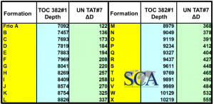
Table 1: Δd for a series of Frio markers in the UN TAT7 well measured against the reference well TOC 382#1
With wells that are properly correlated, a plot of Δd/d will show all points falling on a line (Figure 1). Changes in slope or breaks in the line can indicate faults or unconformities. When there is a miss-correlation, points will plot off of the line (Horizon 27, Figure 2).
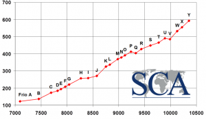
Figure 1: Δd/d plot for the wells shown in Table 1.
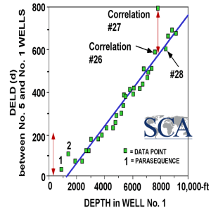
Figure 2: Δd/d plot for wells #1 and 5. Note correlation marker 27 is miss-correlated.
So when you have a lot of previously correlated wells, or mud log or scout ticket data, enter the tops into a spreadsheet, which is an industry best practice in its own right, then calculate and plot Δd. It will help you validate the existing correlations relatively quickly.
Reference:
Bishke, R. E., 1994, interpreting sedimentary growth structures from well log and seismic data (with examples): American Association of Petroleum Geologists Bulletin, v. 7, p 873 – 892
Editor’s Note: To learn more about Δd/d and other tools, methods, and techniques to help ensure accurate subsurface maps, register for SCA’s signature course Applied Subsurface Geologic Mapping. Visit scacompanies.com to learn more about SCA’s training Program and other services, or to read more of the 10 Habits of Highly Successful Oil Finders.
Habit 6B
Bob Shoup and Dan Tearpock
SCA receives many queries about the “The Ten Habits of Highly Successful Oil Finders“. Since applying the best practices that are the foundation of the 10 Habits will help you, or your company, reduce the number of dry holes you drill, SCA has written a column elaborating each of the Habits. Here is the column for Habit 6b.
Successful oil finders ensure that their cross sections are balanced in order to confirm that their interpretations are reasonably correct
Cross sections are an excellent tool to help an interpreter resolve correlation problems, understand the nature of the reservoir distribution, and to ensure the three-dimensional validity of the interpretation. With the exception of correlation sections which are used to help an interpreter make consistent correlations, cross sections must be balanced. Of course, this assumes interpreters are making cross section in the first place. Unfortunately many interpreters do not make cross sections. As we teach around the world, we find that less than half of our students have ever made a cross section.
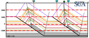
If you recall our discussion of Habit 2 we discussed the story of a veteran geophysicist who had almost 20 years of experience exploring in and mapping growth fault related plays and prospects in the Gulf of Mexico. When he was transferred to a fold and thrust belt region he mapped the key faults with listric geometry and the folds similar to extensional hanging wall rollovers (Figure 1). This resulted in a series of dry holes that led to a costly lawsuit. In the trial, the seismic interpretation and maps were found to have over 100 mistakes and mis-ties.
These mistakes could easily have been avoided if the interpreter had made a cross section across his maps. It would have been quickly apparent that the cross section was not balanced and, therefore, the maps were not valid. Cross sections across compressional structures must be balanced to be valid (Figure 2).
The kinematic relationship between compressional folds and the faults that form them are well understood. There are a number of nomograms and tables available for the interpreter to help them make geologically reasonable interpretations and balanced cross sections. Several of them can be found in Tearpock and Bishke (2003). We highly recommend that interpreters working in compressional fold belts take a structural geology class to familiarize themselves with these kinematic relationships and to learn the appropriate methods needed to ensure valid interpretations and maps. The cost of a class is a few thousand dollars. The cost of a dry hole is a few tens of millions of dollars. And for our interpreter discussed above, the cost of not learning how to interpret and map compressional folds was his career.
But what about cross sections across extensional or diapiric structures, must they be balanced? Since material can flow or slide out of the plane of the section, or the structures are connected to a downdip compressional toe structure, cross sections across extensional folds need not be balanced. However, there are methods that interpreters can use to make geologically and geometrically valid cross sections across extensional structures.
One method is to maintain interval thickness. Whereas individual sands may exhibit marked changes in thickness over short distances, depositional sequences generally thicken or thin gradually, such that they appear to maintain a relatively consistent thickness over large distances. Only when a sequence is impacted by syndepositional growth faults or it has been eroded by an unconformity will it exhibit a large variation in thickness in a short distance.
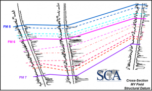
Interpreters can use this understanding to make or review stratigraphic correlations For example the cross section in Figure 3 was constructed by entering the existing correlations in a large field. Note that there are two places on the section where the interval thickness changes, between Formation 6 and 6a between the two left-most wells, and between Formation 6e and 7, also between the two left-most wells.
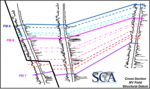
The interval thickness change between Formation 6 and 6a indicates a miscorrelation. Formation 6a is a coal bed. In the middle well, the coal was picked too high; shifting the correlation down to the next coal maintains a constant interval thickness for that sequence (Figure 4).
The interval thickness changes between Formation 6e and 7 are the result of the original interpreter missing a fault in the left-most well (Figure 4). You can see in the final interpretation that the interval thickness between all of the formations is reasonably consistent, although there is some thickening of the Formation 6 horizons into the fault.
As with compressional structures, the kinematic relationship between extensional hanging wall folds and the faults that form them are also well understood. Interpreters can measure the change in dip along a fault and use a nomogram to determine the dip rate of the front limb of the fold.
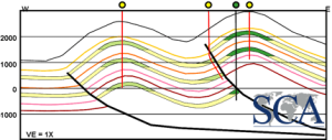
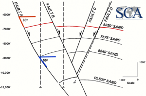
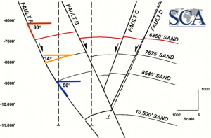
For example, the cross section shown in Figure 5 was constructed from a series of horizon structure and fault surface maps for a prospect in which several wells have been proposed, two vertical and one deviated. We can examine the cross section and see that it looks reasonable, suggesting that the maps that the cross section was drawn from are valid. We can see that the interval thickness does change slightly across the section, however, Fault A is a growth fault, and some thickening into the fault is expected.
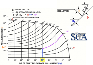
Before we spend millions of dollars drilling three wells into this prospect, we can take an additional hour of our time to validate the maps by looking at the dip portrayed in the front limb of the fold to see if it is correct. We will use the 7675 Foot Sand as our test. Since the cross section was constructed with no vertical exaggeration, we can measure the dip of the fault directly from the cross section. The dip of the fault above the 7675 Foot Sand (β, Figure 6) is 60o and below the sand (α1, Figure 6) it is 50o. The difference is 10o (Ф, Figure 6).
Using the nomogram shown in Figure 6, we can determine that the front limb dip (θ, Figure 6) of the 7675 Food Sand should be 14o. Measuring the dip of the 7675 Foot Sand on the cross section (Figure 7), we see that it is 14o, thereby validating our maps.
Cross sections are an invaluable tool for helping establish and validate correlations, understanding the depositional environment and reservoir distribution, and for confirming the three-dimensional validity of our structural interpretations and maps. Are you making them?
Reference:
Tearpock, D.J. and Bischke, R. E., 2003, Applied Subsurface Geological Mapping with Structural Methods, 2nd Edition, L. G. Walker, editor, Prentice Hall PTR, Upper Saddle River, New Jersey
Editor’s Note: To learn more about cross section construction and other tools, methods, and techniques to help ensure accurate subsurface maps, register for SCA’s signature course Applied Subsurface Geologic Mapping.
Figure Captions:
- Improper interpretation of an imbricate fault propagation fold
- Balanced cross section across the same imbricate fault propagation fold seen in Figure 1
- Cross section across MY Field Formation correlations inherited from the operator
- Cross section across MY Field Formation correlations corrected to maintain constant interval thickness
- Cross section across a prospective structure showing fault dip above and below the 7675’ Sand Dashed lines are proposed well locations
- Nomogram for determining the front limb dip of a hanginng wall anticline (Tearpock and Bishke, 2003)
- Cross section across a prospective structure showing dip of the 7675’ Sand Dashed lines are proposed well locations