Habit 5: Exploring the 10 Habits

SCA receives many queries about the “The Ten Habits of Highly Successful Oil Finders“. Since applying the best practices that are the foundation of the 10 Habits will help you, or your company, reduce the number of dry holes you drill, SCA has written a column elaborating each of the Habits. Here is the column for Habit 5.

Successful oil finders ensure that their seismic and well correlations are accurate and loop-tied.

In our last column we addressed the failure to make accurate well log correlations and the failure to correlate the whole well log, a significant cause of dry holes. In this blog, we will address the failure to make accurate loop-tied seismic correlations which result in inaccurate maps which lead to unnecessary dry holes.

Assumptions

Whenever we are interpreting seismic, whether it is 2D or 3D seismic, we make a number of assumptions, whether we are aware of them or not. Our first assumption is that the data being used are of reasonable quality and have been correctly processed and loaded. The second assumption is that the two-way time to depth conversion is known through our deepest mapped horizon. Finally, we assume we have interpreted the seismic lines correctly. More often than not, one or more of these assumptions is incorrect, so it is up to the interpreter to remain diligent regarding all of these assumptions.

Interpretation Workflow

One way to help ensure accurate seismic interpretations and to avoid interpretation pitfalls, is to have a workflow that helps ensure you apply industry best practices and the 10Habits. We find it useful to follow these steps:

• Before beginning your interpretation, double check that the wells and seismic lines or the 3D survey have been loaded correctly.
• Scale the lines to have close to a 1:1 aspect ratio then scroll through the data set and review the data to determine the structural style and data quality. Switch back and forth from a traditional color bar and a color bar that highlights amplitudes; threshold this color bar to highlight only extreme amplitudes. Note and document any ‘FLTs’, funny looking things.
• Once you have scrolled through the data set, tie the well control to the data, noting faults as well as key horizons encountered in the wells. Make sure that the well ties fit the data. If not, return to step 1.
• Interpret the faults and map the fault surfaces. Review the fault surface maps and make sure that they are geologically reasonable.
• Interpret and map the key horizons. Be sure to loop tie your lines. If you use the workstation for auto picking, ensure that the correlations are consistent by checking to see that the correlations loop tie.
• Create fault polygons for the interpreted horizons. Integrate the horizon maps with the fault surface maps to generate accurate fault polygons where needed.
• Generate amplitude and seismic attribute maps. Ensure any prospective amplitude or attribute anomalies conform to geologic structure, or that they are situated within a geologically valid trap.
• Review the list of funny looking things and see if any are indicative of potential hydrocarbons or prospects.

Loop tying

One tremendous advantage of seismic data is the ability to loop tie our correlations to ensure we are consistently picking the same fault or horizon from line to line. Failure to loop tie will result in miscorrelation of a horizon or aliasing faults; that is connecting two separate faults as one. This often results in the mapping of a screw fault, which is geologically impossible except in strike-slip or structural inversion settings (See Habit 1).

Traps defined by aliased faults are almost always dry holes waiting to happen, such as the case illustrated below in Figure 1. The interpreters picked every 10 cross-lines of the 3D survey to define the structure. The interpreters avoided using in-lines as they were acquired parallel to the strike of the faults, and the “faults were difficult to interpret on the in-lines”.The interpreters defined three principal faults (Faults 1, 2, and 3, Figure 1), with fault 1 interpreted as a bifurcating fault with two splays (1a, and 1 b). Two production platforms can be seen on the map.  Platform A is producing from a closure downthrown to Fault 2. Two wells from Platform B were drilled as long-reach wells to produce from the closure upthrown to Fault 3 and another well was drilled into the closure upthrown to Fault 1. Since that well proved the fault block to be productive, Platform B was installed to produce that block and the block upthrown to Fault 1b.

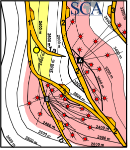
Figure 1: Depth Structure Map, original interpretation

The interpreters defined a small closure downthrown to Fault 1 and upthrown to Fault 1a and a well from Platform B was planned to drain this fault closure (yellow dot, Figure 1). When the well was drilled, the reservoir was encountered at the predicted depth but only had gas shows. In the subsequent post-mortem audit, the reviewers loop-tied the fault picks and mapped the fault surfaces, demonstrating that Fault 1 was not a single fault but two separate en echelon faults (Figure 2). The closure targeted by the well did not exist; and the drilled well was an avoidable dry hole.

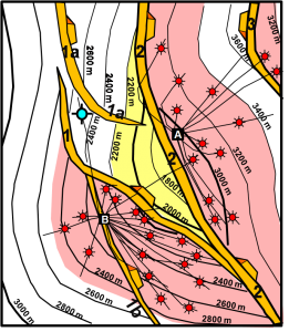
Figure 2: Depth Structure Map, post-audit interpretation

The original map (Figure 1) also suffered from incorrectly mapping through a major fault shadow associated with Fault 2. The structural high in the fault block downthrown to Faults 1 and 1a was mapped as a downthrown fault closure against Fault 1 and 1a. Using restored fault tops and proper mapping techniques such as contour compatibility, the review team was able to demonstrate that the actual structure was an upthrown closure against Fault 2 (Figure 2).

Fault shadows can cause significant challenges to mappers in that they distort the seismic events upthrown to faults. Fault shadows are created when an anisotropic formation, usually a shale, crosses a fault. The fault shadow can be recognized as a zone of distorted seismic below the downthrown intersection of the anisotropic formation and the fault. The zone of distortion can usually be defined by a vertical line (Figure 3).

In the example shown in Figure 3, we can see a compound fault shadow. The first fault shadow, shown by the green dashed line, is set up when the blue horizon (~1.0 sec) crosses the green fault. The second fault shadow (blue dashed line), is set up where the blue horizon crossed the blue fault. Another fault shadow can be observed along the eastern edge of the line where the blue horizon crosses the purple fault.

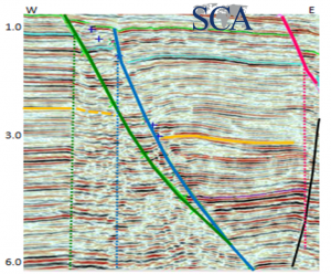
Figure 3: Example of a fault shadow associated with an anisotropic layer crossing a fault

Incorrectly mapping across fault shadows can result in dry holes, such as the one Illustrated above, or in missed opportunities when upthrown traps are miss-mapped as non-closed structures.

There are several methods an interpreter can use to avoid miss-mapping across fault shadows. The most reliable method is to use restored tops when you have wells that cross the fault. In the absence of wells, one can map the upthrown block only up the line of the fault shadow (dashed green line Figure 3). Secondly, map the downthrown block, which is not impacted by the fault shadow. Finally, using the concepts of contour compatibility and vertical separation, one can complete the contours through the fault shadow.

Editor’s Note: To learn more about seismic interpretation register for SCAs Mapping Seismic Data Workshop. To learn more about subsurface mapping and the concepts of contour compatibility and vertical separation, register for SCA’s signature course Applied Subsurface Geologic Mapping. Visit www.scacompanies.com to learn more about SCA’s training Program and other services, or to read more of the 10 Habits of Highly Successful Oil Finders.